Power BI: Summe berechnen


Power BI Meisterklasse: Summe berechnen leicht gemacht
In diesem Beitrag widmen wir uns einem der grundlegenden Elemente in Power BI: der Summenberechnung. Egal, ob du gerade erst beginnst oder bereits ein erfahrener Anwender bist, das Verständnis und die effektive Anwendung von Summenberechnungen sind entscheidend. Wir starten mit einer detaillierten Betrachtung der SUM und SUMX Funktionen und gehen dann über zu verschiedenen Anwendungsszenarien. Weiterhin beleuchten wir, wie du Bedingungen in deine Summenformeln integrieren kannst und schließen mit Strategien zur Optimierung dieser Berechnungen bei umfangreichen Datensätzen ab.
Einführung in SUM und SUMX Funktionen
In unserem heutigen Deep Dive befassen wir uns mit den essenziellen Werkzeugen der Summenberechnung in Power BI: den SUM und SUMX Funktionen. Diese Funktionen sind zentral für die Datenaggregation und bieten vielfältige Anwendungsmöglichkeiten. Wenn du dich gerade am Anfang befindest und dich im Power BI Kosmos noch nicht auskennst, können unsere Power BI Trainings eine echte Stütze sein, um die Grundlagen zu erlernen und Power BI erfolgreich in deinem Unternehmen zu integrieren.
Beginnen wir mit der SUM-Funktion. Diese ist deine erste Anlaufstelle, wenn es um die Berechnung von Summen über eine einzelne Spalte in deiner Datenquelle geht. Die SUM-Funktion ist besonders effektiv, wenn du eine schnelle und unkomplizierte Aggregation von Werten benötigst. Sie ist ideal für Szenarien, in denen du die Gesamtsumme von Elementen wie Verkaufszahlen, Ausgaben oder anderen numerischen Werten ermitteln möchtest.
Stell dir vor, du hast eine Tabelle mit täglichen Verkaufszahlen. Um die Gesamtverkaufszahlen für einen bestimmten Zeitraum zu ermitteln, kannst du einfach die SUM-Funktion auf die entsprechende Spalte anwenden:
SUM(Verkaufstabelle[Verkaufszahlen]
Dieser Ausdruck summiert alle Werte in der Spalte „Verkaufszahlen“ der Tabelle „Verkaufstabelle“. Aber was passiert, wenn deine Anforderungen über einfache Aggregationen hinausgehen?
Hier tritt die SUMX-Funktion in den Vordergrund. SUMX gehört zu den Iterator-Funktionen und bietet eine erweiterte Flexibilität, indem sie es dir ermöglicht, individuelle Berechnungen für jede Zeile deiner Tabelle durchzuführen, bevor die Summe gebildet wird. Diese Funktion ist besonders nützlich, wenn du komplexe Berechnungen über mehrere Spalten oder Tabellen hinweg durchführen musst. Mit SUMX kannst du beispielsweise eine bedingte Logik anwenden, um Summen basierend auf spezifischen Kriterien zu berechnen, oder Berechnungen durchführen, die auf Werten aus mehreren Spalten basieren.
Nehmen wir an, du hast eine Tabelle mit Produkten, deren Preisen und verkauften Mengen. Du möchtest den Gesamtumsatz berechnen. Hier kommt SUMX ins Spiel:
SUMX(Verkaufstabelle, Verkaufstabelle[Menge] * Verkaufstabelle[Preis])
In diesem Beispiel multipliziert SUMX für jede Zeile in der Tabelle „Verkaufstabelle“ die gekaufte Menge mit dem dazugehörigen Preis und summiert anschließend diese Werte. Dies ermöglicht eine zeilenweise Berechnung, die über die einfache Summierung hinausgeht.
Der entscheidende Vorteil von SUMX gegenüber der einfachen SUM-Funktion liegt hier in der Genauigkeit der Berechnung. Mit SUMX berechnest du für jedes verkaufte Produkt im ersten Schritt den Gesamtpreis (Menge * Produktpreis). Erst am Ende bezieht Power BI die Summe über alle diese Gesamtpreise. Dieser Ansatz berücksichtigt die individuellen Preise jedes Produkts in jeder Transaktion, was eine präzise Umsatzberechnung ermöglicht.
Würdest du stattdessen nur die SUM-Funktion verwenden, könntest du zwar die Gesamtmenge aller verkauften Produkte summieren, müsstest diese dann aber mit einem einheitlichen Preis multiplizieren. Dies würde nicht die tatsächlichen Verkaufsbedingungen widerspiegeln, da du nicht für jedes Produkt den spezifischen Preis nutzen könntest. Die Verwendung von SUMX in Power BI ermöglicht daher eine genauere Methode zur Umsatzberechnung, die die individuellen Preise und verkauften Mengen jedes Produkts berücksichtigt.
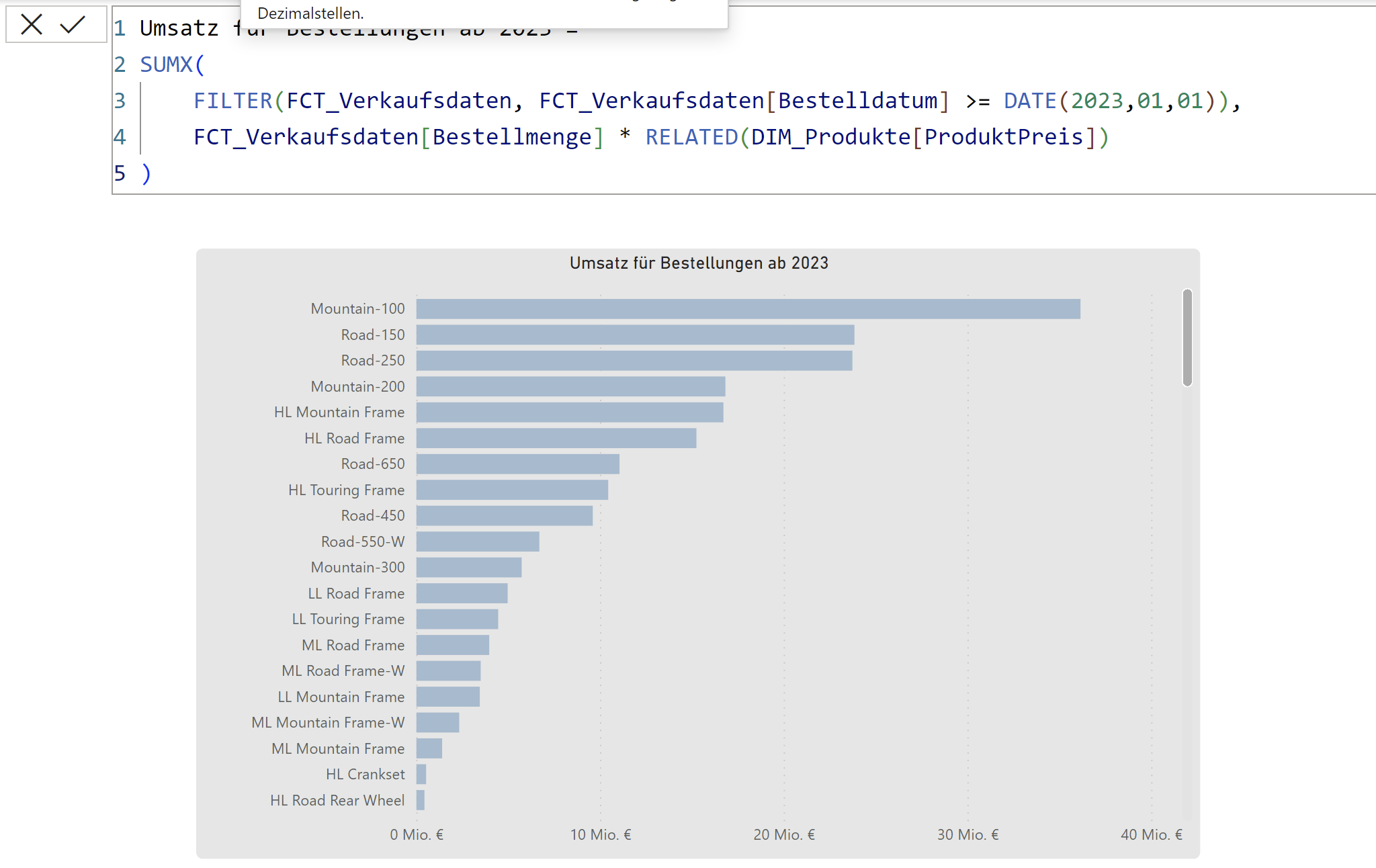
Die Flexibilität von SUMX zeigt sich auch in komplexeren Szenarien. Angenommen, du möchtest den Gesamtumsatz nur für Produkte berechnen, deren Preis über 50 Euro liegt. Mit SUMX kannst du diese Bedingung direkt in die Berechnung einfließen lassen:
SUMX( FILTER(Verkaufstabelle, Verkaufstabelle[Preis] > 50), Verkaufstabelle[Menge] * Verkaufstabelle[Preis])
Hier filtert die Funktion FILTER zuerst die Tabelle, um nur Zeilen mit einem Preis über 50 Euro zu berücksichtigen, und SUMX berechnet dann den Gesamtumsatz basierend auf dieser gefilterten Tabelle.
Ein wesentlicher Unterschied zwischen SUM und SUMX liegt in ihrer Arbeitsweise: Während SUM direkt auf eine einzelne Spalte angewendet wird und die Werte in dieser Spalte summiert, ermöglicht SUMX eine detailliertere Berechnung. SUMX nimmt eine Tabelle und eine Ausdrucksformel entgegen, wodurch es möglich wird, Berechnungen zeilenweise durchzuführen, bevor die Ergebnisse summiert werden. Diese Möglichkeit zur zeilenbasierten Berechnung ist das Kernmerkmal, das SUMX von SUM unterscheidet und es zu einem mächtigen Werkzeug in deinem Power BI Toolkit macht, insbesondere für die Analyse komplexer Datensätze. Die zusätzliche Flexibilität, die durch die Verwendung von Ausdrucksformeln geboten wird, ist ein weiterer Vorteil, der SUMX besonders wertvoll für fortgeschrittene Datenmanipulationen und -analysen macht.
In den folgenden Abschnitten werden wir uns ansehen, wie du diese Funktionen in verschiedenen Szenarien anwenden kannst, um tiefergehende Einblicke in deine Daten zu gewinnen und deine Analysefähigkeiten auf die nächste Stufe zu heben.
Unterschiedliche Anwendungsszenarien für Summenberechnungen
Nachdem wir uns mit den Grundlagen der SUM und SUMX Funktionen vertraut gemacht haben, wollen wir nun einige spannende Anwendungsszenarien anschauen. Summenberechnungen in Power BI sind weit mehr als nur ein Werkzeug für Finanzberichte. Sie bieten vielfältige Möglichkeiten, um tiefere Einblicke in verschiedene Datentypen zu erhalten. Beispielsweise:
Zeitbasierte Aggregationen:
Ein klassisches Anwendungsszenario ist die zeitbasierte Aggregation. Stell dir vor, du verfügst über eine Datenreihe mit monatlichen Energieverbrauchswerten. Mit der SUM-Funktion kannst du den Gesamtverbrauch für ein ganzes Jahr oder einen bestimmten Zeitraum berechnen. Dies hilft dir, saisonale Muster und Trends zu identifizieren.
Für den Fall, dass du eine Tabelle mit den monatlichen Energieverbrauchswerten eines Unternehmens hast, ermöglicht dir die SUM-Funktion, den Gesamtverbrauch für das Jahr zu ermitteln. Die Formel könnte dabei so aussehen:
SUM(Energieverbrauchstabelle[Jahresverbrauch])
Erweiterung für die Kostenberechnung: Nehmen wir nun an, deine Tabelle enthält nicht nur die monatlichen Energieverbrauchswerte, sondern auch die jeweiligen Energiepreise für jeden Monat. In diesem Fall möchtest du vielleicht die Gesamtkosten des Energieverbrauchs für das Jahr berechnen, wobei jeder Monat mit einem anderen Preis bewertet wird. Hier kommt die SUMX-Funktion ins Spiel, die es dir ermöglicht, eine zeilenweise Berechnung durchzuführen, indem für jeden Monat der Verbrauch mit dem entsprechenden Preis multipliziert wird, bevor die Ergebnisse summiert werden. Die Formel könnte wie folgt aussehen:
SUMX(Energieverbrauchstabelle, Energieverbrauchstabelle[Monatsverbrauch] * Energieverbrauchstabelle[Preis pro Einheit])
Durch die Verwendung von SUMX kannst du die Gesamtkosten des Energieverbrauchs präzise berechnen. Das ermöglicht eine detaillierte Analyse der Energiekosten über das Jahr hinweg und hilft dir, die Auswirkungen von Preisänderungen sowie Verbrauchstrends zu verstehen.
Inventarmanagement:
Im Bereich des Inventarmanagements spielen analytische Funktionen eine entscheidende Rolle bei der Bewertung des Gesamtwerts des Lagerbestands oder der Berechnung der durchschnittlichen Lagerdauer von Produkten. Diese Analysen sind von großer Bedeutung für die Optimierung der Lagerhaltung und die Minimierung von Lagerkosten.
Angenommen, du möchtest zunächst den Gesamtwert einer bestimmten Produktkategorie in deinem Lager bestimmen. Wenn deine Tabelle die Anzahl der Einheiten jeder Produktkategorie enthält und du einen einheitlichen Wert pro Einheit über alle Produkte hinweg annimmst, könntest du die SUM-Funktion verwenden, um die Gesamtanzahl der Einheiten zu berechnen:
SUM(Lagerbestandstabelle[Bestand])
Anschließend würdest du dieses Ergebnis mit dem einheitlichen Wert pro Einheit multiplizieren, um den Gesamtwert des Lagerbestands für diese Kategorie zu ermitteln. Diese Methode bietet jedoch nur eine grobe Schätzung, da sie von einem einheitlichen Preis pro Einheit ausgeht.
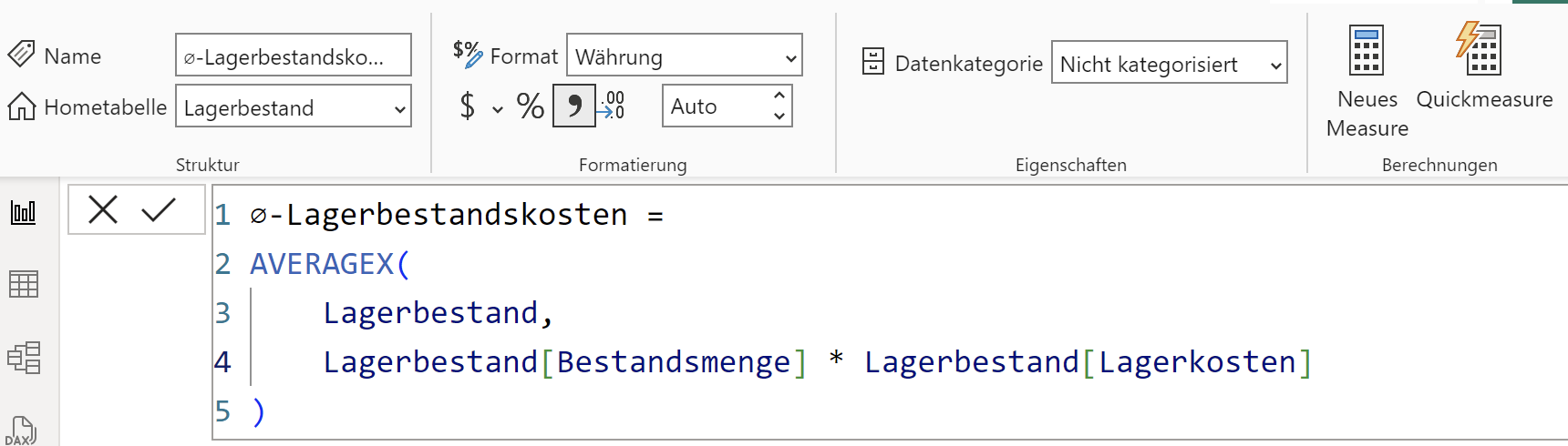
Für eine genauere Berechnung, die unterschiedliche Werte pro Einheit berücksichtigt, ist die SUMX-Funktion ideal. Nehmen wir an, deine Tabelle enthält nicht nur den Bestand, sondern auch den spezifischen Wert pro Einheit für jedes Produkt. Mit SUMX kannst du den Gesamtwert des Lagerbestands präziser ermitteln, indem du für jedes Produkt im Lager den Bestand mit dem jeweiligen Wert pro Einheit multiplizierst und diese Produkte dann summiert:
SUMX( Lagerbestandstabelle, Lagerbestandstabelle[Bestand] * Lagerbestandstabelle[Wert pro Einheit])
Diese Methode ermöglicht eine detaillierte Bewertung des Lagerbestands, indem sie die spezifischen Werte pro Einheit jedes Produkts berücksichtigt. Sie ist besonders nützlich für Inventarmanagementaufgaben, bei denen Produkte mit unterschiedlichen Preisen und in verschiedenen Mengen vorliegen. Durch die Anwendung von SUMX können Unternehmen eine genauere Einschätzung ihres Lagerbestandswerts erhalten, was wiederum eine effizientere Lagerhaltung und Kostenreduktion unterstützt.
Diese Beispiele zeigen, wie vielseitig SUM und SUMX in Power BI eingesetzt werden können. Sie ermöglichen es dir, aus deinen Daten wertvolle Erkenntnisse zu gewinnen, die weit über einfache Summen hinausgehen und dir helfen, fundierte Entscheidungen in verschiedenen Geschäftsbereichen zu treffen.
Integration von Bedingungen in Summenformeln
Die wahre Stärke von Power BI zeigt sich, wenn es darum geht, nicht nur einfache Summen zu berechnen, sondern auch spezifische Bedingungen in diese Berechnungen zu integrieren. Anstatt SUMIF und SUMIFS, die in Excel verwendet werden, bietet Power BI leistungsstarke DAX-Funktionen wie CALCULATE und FILTER, um bedingte Summen zu berechnen. Mehr zu den Funktionen CALCULATE und FILTER findest du in unserem Blogbeitrag “5. Power BI: Kumulierte Werte berechnen”.
Bedingte Summenbildung mit CALCULATE und FILTER:
Diese Kombination ermöglicht es, Summen für Datensätze zu berechnen, die bestimmte Kriterien erfüllen. Stell dir vor, du hast eine Tabelle mit Verkaufsdaten und möchten den Gesamtumsatz nur für ein bestimmtes Produkt berechnen. Du kannst dies mit einer Kombination aus CALCULATE und FILTER erreichen:
CALCULATE( SUM(Verkaufstabelle[Umsatz]), Verkaufstabelle[Produkt] = "Produkt A")
In diesem Beispiel summiert CALCULATE den Umsatz in der Tabelle „Verkaufstabelle“, aber nur für Zeilen, in denen das Feld „Produkt“ den Wert „Produkt A“ hat.
Erweiterte Anwendungen mit Mehrfachkriterien:
Für komplexere Szenarien, in denen du Summen basierend auf mehreren Kriterien berechnen möchtest, kannst du die FILTER-Funktion innerhalb von CALCULATE erweitern. Angenommen, du möchtest den Gesamtumsatz für ein Produkt in einer bestimmten Region und innerhalb eines bestimmten Zeitraums ermitteln:
CALCULATE( SUM(Verkaufstabelle[Umsatz]), FILTER( Verkaufstabelle, Verkaufstabelle[Produkt] = "Produkt A" && Verkaufstabelle[Region] = "Region 1" && Verkaufstabelle[Verkaufsdatum] >= DATE(2023, 1, 1) && Verkaufstabelle[Verkaufsdatum] <= DATE(2023, 12, 31) ))
Hier summiert CALCULATE den Umsatz für „Produkt A“ in „Region 1“, aber nur für Verkäufe, die im Jahr 2023 getätigt wurden.
Diese Beispiele zeigen, wie du mit DAX-Funktionen wie CALCULATE und FILTER gezielt Daten aggregieren kannst, die bestimmten Bedingungen entsprechen. Diese Methoden sind extrem nützlich, um spezifische Einblicke aus deinen Daten zu gewinnen und fundierte Entscheidungen auf Basis präziser Datenanalysen zu treffen.
Optimierung von Summenberechnungen für große Datensätze
Die Arbeit mit großen Datensätzen in Power BI kann herausfordernd sein, insbesondere wenn es um effiziente Summenberechnungen geht. Große Datenmengen erfordern eine sorgfältige Planung und Optimierung, um Performance-Einbußen zu vermeiden. Hier sind einige fortgeschrittene Strategien, um deine Summenberechnungen auch bei umfangreichen Daten effizient zu gestalten:
- Effiziente Datenmodellierung: Nutze „Star Schema“ oder „Snowflake Schema“ und integriere nur relevante Daten, um die Verarbeitung zu beschleunigen.
- Intelligente Berechnungen: Setze auf vorberechnete Spalten und berechne Zwischenergebnisse im Voraus, um die Rechenlast zu minimieren.
- DAX-Funktionen: Nutze DAX-Funktionen wie CALCULATE für effiziente Summenberechnungen mit komplexen Filterlogiken.
- Inkrementelles Laden: Lade nur neu hinzugekommene oder geänderte Daten, um die Performance zu steigern.
- Überwachung und Tuning: Identifiziere und behebe Engpässe mit Performance-Analyse-Tools in Power BI.
Diese Maßnahmen helfen, Summenberechnungen auch bei umfangreichen Datenmengen effizient durchzuführen und die Leistungsfähigkeit von Power BI optimal zu nutzen.